Analyzing rail grinding patterns
Written by Jenifer Nunez, assistant editor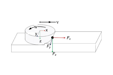
Rail grinding management is an important part of a railroad's maintenance practices, with an end goal of giving rail the longest life-cycle possible.
Rail grinding management is an important part of a railroad’s maintenance practices, with an end goal of giving rail the longest life-cycle possible.
As railroads continue to improve their rail grinding practices and take advantage of new technologies in rail profile inspection and grinding train control systems, as well as improved understanding of the wheel/rail interface relationship, it becomes increasingly important for grinding control systems to be able to effectively analyze the performance of different grinding patterns in a real world operating setting. This has led to different efforts to model the rail grinding process, both individually, as a function of a single grinding motor on the head of the rail, and in the more complex configuration of multiple grinding motors in a range of patterns. Thus, for a 96 stone grinding train with 48 motors per rail, it is necessary to analyze the full sequence of 48 motors as each motor individually and sequentially removes metal from the rail head. Furthermore, this analysis must be sensitive to key factors, such as grinding speed and the key pattern parameters of motor angles, sequence and power. The ability to effectively perform this type analysis allows for better management of the grinding process and improved planning of grinding activities. 1, 2
Two approaches are generally available for the analysis of the metal removal on the rail head.
The first approach makes use of a “closed form” mathematical representation of the rail head, where the shape of the rail head is defined according to the design radii (per AREMA standard rail profile design drawings).
The second approach makes use of a digitized rail profile, such as taken from a modern rail profile measurement system.
In both cases, it is necessary to first define the three dimensional coordinate system of the grinding wheel moving along the axis of the rail head, as shown in Figure 1.
Figure 2 shows the rail cross-section (as defined by the three radii per AREMA drawings) with a grinding stone located at the motor position angle.
Assuming that the rail profile can be accurately characterized by a continuous mathematical function (an assumption that becomes more questionable as the rail wears and assumes a non-uniform profile), then the effect of a single grinding stone can be calculated as a function of the grinding angle, as shown in Figure 3.
As it has been well documented,2 the actual length of the cut (the facet width) varies directly with the angle of the grinding motors. Using a defined metal removal volume per unit of time (such as can be obtained from a laboratory grinding motor test measuring total metal removal per unit time), it is possible to calculate the associated cross sectional area of metal removal as a function of the forward speed of the grinding train. This, in turn, allows for the calculation of the depth of cut as a function of the contact length (facet width) and speed of the train. Figure 4 shows the relationship between the grinding angle and contact lengths (facet width). Note, as expected, the contact length decrease as the motor angle increases. However, as the contact length decreases, there is a corresponding increase in the cutting depth to maintain a constant area of metal removal (for a fixed grinding speed).
However, as already noted, the ability to define a worn rail profile as a continuous function is difficult. A more practical approach is to use the x-y coordinate profile array developed directly from a modern rail profile measurement system, 1,2 such as shown in Figure 5 for a pre-grind and post grind rail profile.
Using these digitized profiles, it is then possible to analyze the metal removal by an individual grinding wheel using a three step iterative process as follows:
•Find the peak point first (find the furthest point to this orientation line based on the motor angle).
•Cutting step by step into the rail head with set grinding capability (e.g. selected area increment).
•Based on the first cut result, adjust the contact position of the grinding stone and begin the second iteration.
Thus the grinding process can be considered to be a series of individual cutting lines, moving into the rail head and removing the rail head area located above the cutting line. Intersecting points can be found as the cutting line “cuts” through the rail profile. The total removed area can then be calculated by accumulating all the area above the cutting line. When this area equals the metal removal area calculated for the defined grinder speed, then then calculation is complete for this grinding stone.
Note, again, the shape of the removed area will vary as a function of the shape of the rail profile, the motor angle (position of the grinding stone on the rail profile), the power setting of the motor and as well as the cutting ability of the grinding stone (volume of area removed per unit time).
Once the removal area reaches the defined area removal value level for this stone, the penetration analysis ends and the new “post-grind” profile is generated.
This is the case for one grinding motor (one stone). The next motor in the pattern sequence then starts to cut on the “ground” profile (as opposed to the original rail profile). The effect of this sequence is shown in Figure 7.
Thus, using a sequence of profile calculation of individual grinding stones, a full pattern grinding program can be implemented. Using the sequence of motor angles and power settings, based on the defined grinding pattern, those stones grind the rail profile one by one. The profile ground by the previous stone would be the new profile to be ground for the next one, as shown in Figure 7. This indicates that the grinding pattern effectiveness is not only determined by the cutting capabilities of individual stones, but also significantly impacted by their cutting sequences defined by the grinding pattern.
Using this approach, the effect of a full 48 motor grinding sequence was analyzed using field data obtained by a Harsco high-production 96 motor rail grinder on a Class 1 railroad. Specific pre- and post-rail profile data was available for a range of patterns, speeds and rail conditions, as shown in Figure 5.
Given the high level of accuracy of the profile measurement system used, it was possible to calculate the change in the rail cross-section area due to the rail grinding by directly subtracting the post-grind profile from the pre-grind profile. These values are presented in Table 1, as Area Removed, together with the corresponding per-motor area (A/stone) and the corresponding metal removal volume (Q in cubic inches per minute), which is calculated using the speed of the grinding train (eight mph in the case of Table 1).
As can be seen in this data sample, the calculated value for Q is consistent.
Using these Q values in the grinding model, based on the defined grinding pattern (Pattern 1), good agreement is achieved between the measured post-grind profile (blue) and the calculated post-grind profile (red) as shown in Figure 8.
It should be noted that errors associated with data collection in some of the profiles resulted in zones of missing data, such as seen in Figure 9.
By developing more sophisticated analysis and evaluation tools that allow for more accurate modeling of the grinding process, railroads can continue to improve their rail grinding practices and take further advantage of new technologies in rail profile inspection and grinding train control systems and better manage both the grinding process itself and the planning of grinding activities.
References
1. Zarembski, A.M., “Management of Total Rail Grinding Maintenance Process,” Railway Track & Structures,
June 2011.
2. Zarembski, A.M., The Art and Science of Rail Grinding, Simmons-Boardman Books, Inc., Omaha, Neb.,
August 2005.