Research: Future of Weibull Defects Analysis in the Railway Industry
Written by Ahmed Lasisi
Transportation Safety Board of Canada
Editor’s Note: From time to time we will publish cutting-edge research in the world of rail engineering. In this piece, researchers ponder the possible flaws of Weibull analysis in preventing defect-caused derailments.
Weibull analysis is a significant tool that is heavily relied upon in rail defect analysis[1]. Federal railroad administration-FRA data shows that 30 to 40% of railway accidents are track-related, only second to human causes[2]. A scrutiny of FRA derailment data reveals that rail defect and track geometry are the leading causes of track-caused derailments. While this article is intended to address Weibull and rail defect, we have focused on track geometry in another study[3]. Between 2001 and 2010, two types of defect (transverse fissures and detail fractures) accounted for over 65% of broken-rail-caused derailments, and this proportion increased to approximately 70% in the following years[4]. Hence, why do we still have rail defect-caused derailments around if the Weibull defect analysis has very been effective?
A Glimpse at Applications of Weibull in the Railroad Industry
Although we intend to accommodate all possible audience in the readers’ community, it is very important that we describe the Weibull Analysis to put this discussion in the intended perspective. The cumulative probability of defect occurrence is expressed as a function of the accumulated tonnage (in Million Gross Tons (MGT)) of the rail. A Weibull plot (log-log scale) of the cumulative defect data and the accumulated MGT produces a positive linear relationship.
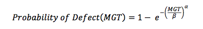
Where: a is the shape parameter or the slope of the line, and β is the scale parameter or characteristic life or Weibull intercept.
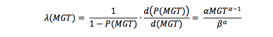
The rate of defect propagation or failure rate is the first derivative of the probability given as λ:
Given this information and the annual track tonnage, T, the cumulative number of defect per mile per year (N) can be computed as follows:
![]()
Where 271 is the number of rails (39ft length) per mile of track.
The life of rail in a track in (MGT) is then computed as follows:
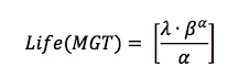
Weibull analysis has been widely applied in the railroads to address defect growth rate and reliability issues. Its application is also found in other track components like ballast, ties, turnouts, track circuits, wheels, axles, etc. Its application has been heavily relied upon for short-term, long-term, and intermediate-term analysis[5]&[6]. With this wide spectrum of application, data science experts can readily spot a flaw because it is impossible for a single statistical technique to perform excellently on all different kinds of data. A more technical way of saying this is: “any two optimization (or machine learning) algorithms are equivalent when their performance is averaged across all possible problems.”[7]. Therefore, something is inherently wrong, not with the Weibull distribution but its ubiquitous application in the railroad industry; and railroad practitioners should not wait until something terrible happens before taking action.
Limitations and Shortcomings
Even though the shortcoming hinted above is very intuitive for the data savvy and professionals in the statistical community, there are other dire limitations and shortcomings. While the Weibull analysis as described above appears very objective and mathematically driven, a crucial element that is often overlooked is that defect data is “condemned” to follow a given distribution: Weibull. Distributions are a good way of describing our data but what should not be misunderstood is that a fitted distribution may not be able to anticipate a data to which it has not been exposed or trained. Hence, like most distributions, they are often trained and tested on the same data. What happens when they are tested on a data not yet seen?
In a data driven age like the one we live in, it is not very intelligent to train and test a distribution or technique on the same dataset. This is like examining students on identical problems already treated as examples in class. Because of this shortcoming, Weibull distribution is not effective at predicting unseen data. Another important issue to be addressed is the overwhelming number of equations to be fitted for different defect types across different sections of track. For example: to do a rigorous defect analysis for all defect types across a mile of track, we assume that the total number of defects are ten (10) even though there are more and that there are 500 miles of track in a given district. Each given defect requires a different equation for every mile of track. A simple estimate shows approximately five thousand Weibull equations to be developed for monitoring rail defects in that district. In today’s world, five thousand equations does not sound like a computational burden but is this approach really an efficient way of analyzing defect?
Possible Improvements
A part of the railroad community admits many of these shortcomings, some are very resistant to change perhaps because they are risk-averse. Others are very honest to openly declare that something needs to be done. The use of a 3-parameter Weibull was thought to be the solution. A 3-parameter Weibull includes a location parameter in addition to the scale and shape parameters previously discussed. The third parameter is an intercept/failure free version which belongs to a more generalized form of beta distribution. Even though some studies show that it does fit better, there is certainly a debate about its use because it cannot be rationalized like the 2-parameter.[8] Within certain communities, rationality is not really an issue as long as accuracy and precision is not compromised. The natural question then is: is the 3-parameter Weibull free of the other shortcomings highlighted above?
In this article, we present possible ways in which the Weibull or defect analysis can be improved in two major ways. We understand that the industry struggles with change and any viable solution to be proffered has to be in cognizance of this fact.
Machine-learning enhanced Weibull analysis is one way to take this leap towards improvement. This approach still takes cognizance of defect analysis based on defect type and section, but it certainly open doors for prognostic analysis and testing on unseen dataset. Mathematically speaking:
a, β and λ are scale, shape and location parameters that are currently learnt using either graphical methods, least square regression, method of moments, maximum likelihood estimation and other modifications of the aforementioned[9]. While these methods are great, many of them are classical and they do not completely address many modern data challenges with unseen data. Machine learning is a popular way to solve this problem. While most railroads talk about machine learning, its application is still very far-fetched. Machine learning is a category of algorithm that enables us to be more accurate in predicting outcomes without being explicitly programmed. The basic understanding is to learn from data and improve performance (prediction) of unseen future data as more and more historical or present data is observed.
One way to improve defect analysis is to learn the Weibull parameters using machine learning so it can be very effective at predicting future data. In other words,
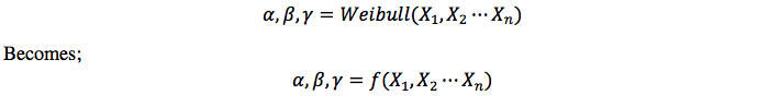
Where f() can be a machine learning function (e.g. support vector machine, random forests, gradient boosting, etc.) that can be selected via several rigorous model selection methods. A good resource for this can be found in[10] while practical illustrations are repose in [11]. Because this is not technical paper, we do not want to bore our readers with too many jargons, hence, the simplicity of the language employed.
The above approach does not necessarily solve the micro-level decision based Weibull defect analysis but it does address the problem of unseen dataset because the trained parameters can then be validated and tested on an unseen dataset. One novel approach to address defect analysis from a network-level is to employ an aggregated learning framework using a matched defect/geometry dataset. Aggregated learning because several machine learning techniques would be able to address the different defect modes in different locations (recall: no free lunch theorem).
Aggregated defect data set because defect growth (or probability) is not only dependent on cumulative tonnage. Rather, other properties, like size of defects, annual tonnage, and presence of geometry defects amongst others are significant factors that contribute to defect growth. This, we found from a study just concluded on rail defect data from a Class 1 railroad. The data consist of a matched rail defect and track geometry datasets spanning over five years with over three hundred thousand geometry exceptions and fifty thousand rail defects. The total length of track observed is about twenty-two thousand miles. It is difficult for an infrastructure owner or manager to plan maintenance allocations using conventional Weibull analysis on this kind of data.
With an aggregated ensemble learning framework, we came up with a tool for macro-level decision making. Before elaborating on the decision-making tool, it is important to introduce the idea of ensemble learning. Ensemble learning stretches further the idea of machine learning but in a democratic way. Rather than rely on a single method (e.g. Weibull, or even Random Forest) to analyze defects, several mediocre learners are brought together. The choice of mediocre or base learners should be as diverse and inclusive as possible so that their individual errors can be uncorrelated. Hence, they complement one another. A simple framework for a multi-step learning ensemble is provided below:
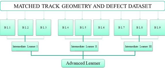
Figure 1: A tree-step framework for analyzing defect data.
The above figure illustrates a simple architecture for learning from rail track data. The first layer represents matched defect and geometry data. That is, from the ocean of data described above, only the sections of track with both geometry exceptions and rail defects were considered so as to include the effect of track geometry on rail life. The second layer represents different base learners or BL that have been trained on the data. While most learners are better that the others, the errors of the best learners can be complemented by the successes of others through an intermediate learning process described in layer 3. The last layer is the advanced learning process where the intermediate learners are combined and insights are comprehensively drawn from the data. While this framework provides a useful guideline, the architecture can be customized to fit specific defect type or analysis.
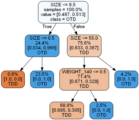
Figure 2: A decision tree for fatigue defect prediction.
A byproduct of the aggregated ensemble learning process is the use of decision trees to formulate rules and influence decision making. A simple rule than can be extracted from Figure 2 is: If the size of other defect types (OTD) is less than or equal to 8.5, and fatigue defects (TDD) has a size is at most 55, and about half of the rails in the network are 140 lb., infrastructure managers should expect about 70% of fatigue defects relative to all other defects in the network.
With this kind of information, managers or infrastructure owners can evaluate their spending and budgets on each defect type and can be sure contractors aren’t demanding for more than required. Because this is not a technical paper we have reserved many of the details found in this study for an appropriate audience elsewhere.
We wrap up this article with an insightful finding from the dataset described. The Weibull along with several variations of the ensemble learning were trained across the aggregated data from the network. The testing was conducted on a data split for high tonnage. It is obvious from Figure 3 that the Weibull overestimates the cumulative probability of defect at high tonnage. While this conservativeness sounds like a precautionary approach, it is actually dangerous. We described above that it is the first derivative of the Weibull that is used for estimating defect not the probability itself. Hence, because the Weibull is climaxing the defect earlier, the derivative or the defect rate is lower, hence lower number of cumulative defects. The implication of this is that there are several defects that are missed. Could this missed defects be the reason from the perpetuity of rail-defect caused derailments in the railroad industry?
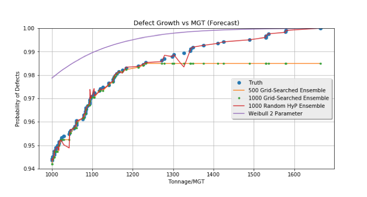
Figure 3: A defect growth forecasting using Weibull and ensemble learning
Concluding Remarks
Weibull-based defect analysis has been around in the railroad industry for many decades and it has significantly influenced the way maintenance decisions have been made. As our engineering problems are evolving, it is expected that our decision making tools are adapted to adequately address our problems. There is no point in being fixated on an ideology if empirical facts clearly suggest otherwise. The fact is that rail-defect-caused derailments remains an issue in this industry but our analytical tools remain fairly unchanged to address the problem.
Machine learning and data science has become a buzzword in the rail industry but very few have adept understanding sufficient enough to harness it. Majority of the folks who are machine learning savvy know nothing about railroads; and the converse is also true. Hence, this article is an attempt to bridge this gap by using an illustrative example in the Weibull as a wake-up call for railroad professionals. Promising results from this and similar studies clearly emphasize the need for further studies on the application of aggregated machine learning in rail defect analysis and other applications in the “rolling-stock” industry.
Acknowledgements
The authors (Ahmed Lasisi and Nii Attoh-Okine, PhD., PE) would like to acknowledge Dr. Allan Zarembski and Engr. Joe Palese for their valuable contributions.
References
[1] A. M. Zarembski, T. L. Euston, J. W. Palese, and C. Hill, “Use of Track Component Life Prediction Models in Infrastructure Management,” AusRAIL PLUS, p. 18, 2005.
[2] FRA, “FRA Office of Safety Analysis,” 2017. [Online]. Available: http://safetydata.fra.dot.gov/officeofsafety/default.aspx.
[3] A. Lasisi and N. Attoh-Okine, “Principal components analysis and track quality index: A machine learning approach,” Transp. Res. Part C Emerg. Technol., vol. 91, no. April, pp. 230–248, 2018.
[4] X. Liu, A. Lovett, T. Dick, M. Rapik Saat, and C. P. L. Barkan, “Optimization of Ultrasonic Rail-Defect Inspection for Improving Railway Transportation Safety and Efficiency,” J. Transp. Eng., vol. 140, no. 10, p. 04014048, 2014.
[5] D. Y. Jeong, “Analytical Modelling of Rail Defects and Its Applications to Rail Defect Management,” Cambridge, MA, 2003.
[6] A. P. Patra and U. Kumar, “Availability analysis of railway track circuits,” Proc. Inst. Mech. Eng. Part F J. Rail Rapid Transit, vol. 224, no. 3, pp. 169–177, 2010.
[7] D. H. Wolpert and W. G. Macready, “No free lunch theorems for optimization,” IEEE Trans. Evol. Comput., vol. 1, no. 1, pp. 67–82, 1997.
[8] A. M. Zarembski, H. Mbr AREMA Nii Attoh-Okine, and P. John Cronin, “Rail Fatigue Life Forecasting Using Big Data Analysis Techniques,” Transp. Res. Board, 2017.
[9] H. S. Bagiorgas, M. Giouli, S. Rehman, and L. M. Al-Hadhrami, “Weibull parameters estimation using four different methods and most energy-carrying wind speed analysis,” Int. J. Green Energy, vol. 8, no. 5, pp. 529–554, 2011.
[10] S. Marsland, MACHINE LEARNING, An Algorithmic Perspective. CRC Press, 2015.
[11] Attoh-Okine, Big Data and Differential Privacy. Wiley Series in Operations Research and Management Science, 2017.